IRLS - Example 1

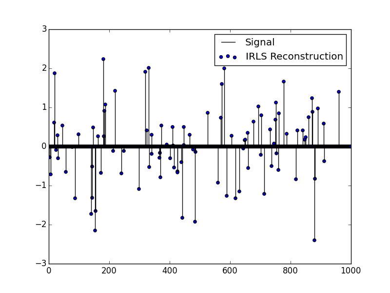
This example is a simple reconstruction of a sparse signal using Lp minimization. We generate a signal, a measurement matrix, and "measure" the signal using the measurement matrix. Using only the measurement matrix and measurement, we reconstruct the original signal.

n=1000   #Signal Dimensions
m=400    #Measurement Dimension
k=100    #Approximate Sparsity

Signal = zeros(n)     #Create a random sparse signal
Signal[int(rand(k)*(n-1)+1)] = randn(k)

MM = randn(m,n)     #Create a random measurement matrix
Measurement = MM*Signal  #Measure the signal using the measurement matrix

#Reconstruct using IRLS
Reconstruction = IRLS(MM,Measurement,verbose=true)

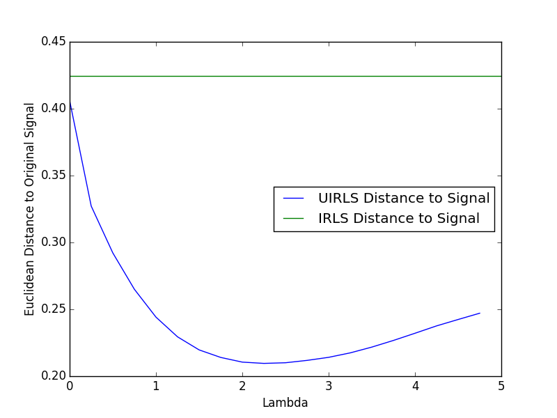
UIRLS w/ Noise - Example 2

Taking the signal and measurement matrix from example 1, we add noise to the measurement and attempt to rebuild the original signal. We then measure the euclidean distance to the true signal, showing that the UIRLS algorithm is superior at rebuilding the signal in the presence of noise.

Noise = randn(m)*.3
Measurement += Noise  #Add ~30% noise to the measurement and reconstruct

#reconstruct using IRLS and UIRLS at multiple lambdas
IRLS(MM,Measurement)
UIRLS(MM,Measurement,lambda=.1)

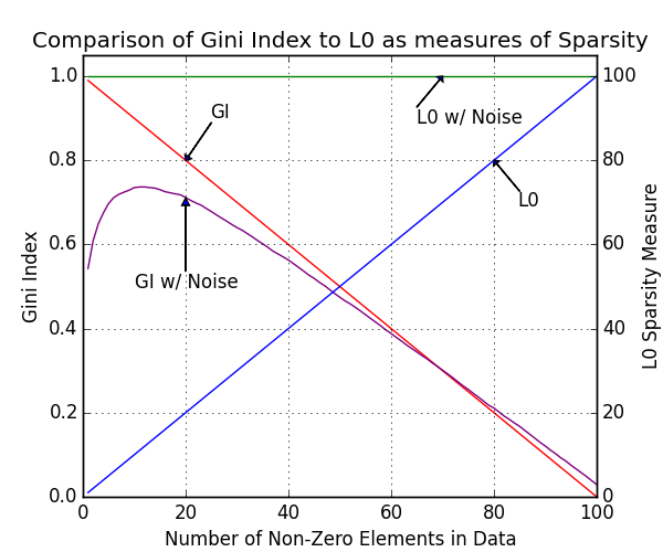
Gini Index - Example 3

The gini index is an excelent measure of the sparsity of a dataset, a full discussion of its benefits are discussed in [4]. To briefly see the benefit, we can look at the difference between GI and L0 as a measure of sparsity on noisy and non-noisy data. Here we have made 2 vectors of length 100, one without noise and one with noise. The noiseless vector starts set to 0, and each element is incrementally set to 1. Taking the L0 sparsity of this, we get the expected result of 1,2,3 etc. However if we add a small amount of noise to the vector, the L0 sparsity is fixed at 100. A comparison to the GI is visible.

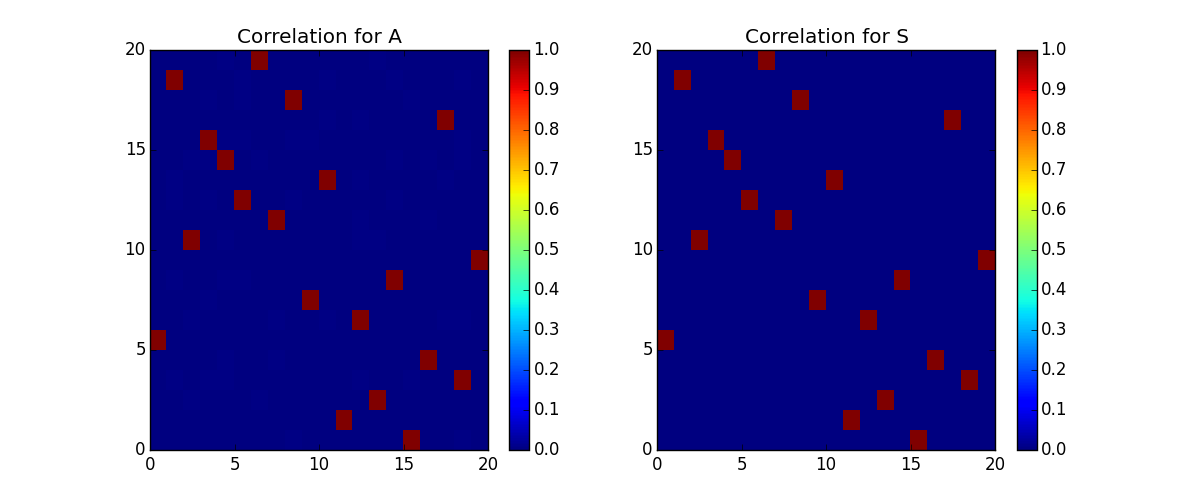
nGMCA- Example 4

The nGMCA algorithm performs blind source separation on a matrix Y, attempting to reconstruct two sparse, non-negative matricies, A, S, that can be mulitplied together such that A*S=Y. Here we make 2 known sparse matricies, A and S, and create a Y. Then using only the Y, we attempt to rebuild A and S with nGMCA. Since the order of rows and columns of A & S can be swapped and scaled and still result in the expected Y, we have to look at the correlation between the reconstructed matricies to the originals in order to see if it found the correct answer.

ZAP - Example 5

The ZAP algorithm attempts to find a jointly-sparse signal M that solves the Multiple Measurement Vector problem described by A * M = Y, where A is a measurement matrix, and Y is the measured signal. A complete discussion of this can be seen in the paper [2]. Figure 1 from that paper is recreated below using this implementation.